Latent Class Growth Analysis and Growth Mixture Modelling
Introduction
Clustering is the task of grouping set of data into subgroups, such that data points within a subgroup (a cluster) is similar to each other but is different from other subgroups. However, clustering algorithm such as K-means clustering does not necessarily consider the temporal aspect of the data.
Growth mixture modelling (GMM) and Latent Class Growth Analysis (LCGA) are two types of longitudional modelling techniques that identify homogenous subpopulations based on growth trajectories. In medical research, the tools can be applied to study the different developmental trajectories within a population.
A useful framework for beginning to understand latent class analysis and growth mixture modelling is the distinction between person-centred and variable-centred approaches. Variable-centred approaches such as regression […] focuses on describing the relationships among variables. The goal is to identify significant predictors of outcomes, and describe how dependent and independent variables are related. Person-centred approaches, on the other hand, include methods such as cluster analysis, latent class analysis, and finite mixture modelling. The focus is on the relationships among indiviudals, and the goal is to classify individuals into distinct groups or categories based on individual response patterns[1].
One example that I am very interested in was this paper by Bandoli et al. [2], where the authors have examine whether patterns of prenatal alcohol exposure differentially affect dysphormic features in infants.
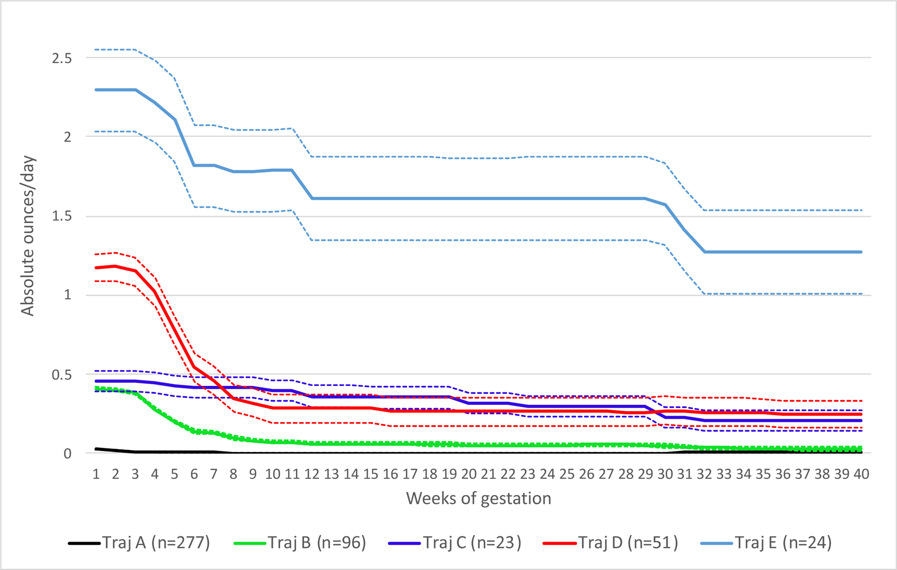
Here, using longitudinal modelling, the authors found 5 distinct trajectories of development, which corresponded to high sustaiend, moderate/high, low/moderate sustained, low/moderate and minimal/no prenatal alcohol exposure. Dysmorphology score was then calculated and examined for association with trajectory of prenatal alcohol exposure.
Example
The following two tutorials explain quite clearly how to carry out LCGA and GMM in R [3,4]. You can also use the following tutorial to generate some simulated data here [5].
Suppose you have a data for 100 cases, each with 5 equally spaced repeated measures on a continuous outcome scale (total of 500 data points).
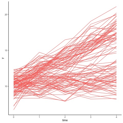
Suppose we are now interested in separating this underlying dataset into sub-populations, where individuals within the same group have very similar trajectories.
In R, both LCGA and GMM can be accomplished with the flemix package. Below is an example with LCGA,
lcga_fit <- stepFlexmix(. ~ .|ID,
k = 1:5,
nrep = 100,
model = FLXMRglmfix(y ~ time, varFix = T),
data = mydata,
control = list(iter.max = 500, minprior = 0))
This code will try out different configurations of the data, and allows us to choose the best fit model. Of interest to us are the following parameters:
- k-> the number of latent subpopulations we want the model to test.
- nrep -> number of random initialisation. Here, the model can find a local minima, but may not be the most optimal output.
In all model configurations, we have fitted y as the dependent variable of time. The error variance is the same in all data groups.
Example output:
| iter | converged | k | Integrated Completed Likelihood |
|---|---|---|---|
| 2 | True | 1 | 2311.291 |
| 5 | True | 2 | 1788.269 |
| 10 | True | 3 | 1784.632 |
| 34 | True | 4 | 1776.328 |
| 29 | True | 5 | 1776.853 |
This table indicates that the model can converge at all 5 different configurations. Using a model fit measure such as the integrated completed likelihood (or Akaike information criterion), we can decide which model we want (here, the lower the score the better). For example, here we can examine the models with two and four latent subpopulations, as the differences between the model fit measures in k=1 and k=2 is most dramatic, and there is not much difference between k=4 and k=5.
The package also allows us to check the posterior probability of the cluster assignments.
| prior | size | post>0 | ratio | |
|---|---|---|---|---|
| Comp.1 | 0.5 | 250 | 265 | 0.943 |
| Comp.2 | 0.5 | 250 | 255 | 0.980 |
| prior | size | post>0 | ratio | |
|---|---|---|---|---|
| Comp.1 | 0.318 | 160 | 250 | 0.640 |
| Comp.2 | 0.234 | 120 | 255 | 0.471 |
| Comp.3 | 0.266 | 130 | 245 | 0.531 |
| Comp.4 | 0.181 | 90 | 230 | 0.391 |
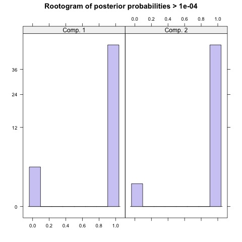
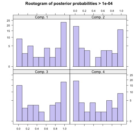
Focusing on the result on the left, the model with two latent subpopulations indicates that equal number of observations were assigned to cluster 1 and cluster 2. Furthermore, the high ratio in either components indicates there is a high confidence of membership. This is, however, not the case for the model on the right. Although the model fit score is lower in this configuration, the rootograms indicate that compared to the first model, this model cannot reliably differentiate between the four clusters.
This is more evident when we plot the cluster memberships for each observation as follows
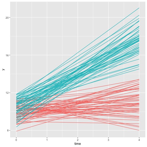
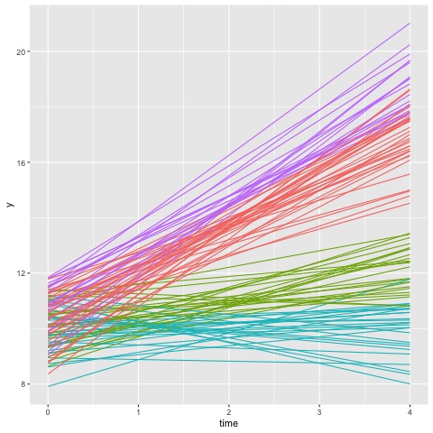
Thus, this suggests that the data would be better fit with a 2 latent population configurations. Next, we can examine whether the cluster membership is associated with any other covariates of interest, such as age, gender or demographic information.
References
[1] Jung and Wickrama. An Introduction to Latent Class Growth analysis and Growth Mixture Modeling
[2] Bandoli et al, 2020. Patterns of Prenatal Alcohol Exposure and Alcohol-Related Dysmorphic Features
[3] https://www.youtube.com/watch?v=cqnpN1k1mPk&ab_channel=RegorzStatistik
[4] https://www.youtube.com/watch?v=sQfIeOh3rJQ&ab_channel=RegorzStatistik
[5] Wardenaar, K. (2020). Latent Class Growth Analysis and Growth Mixture Modeling using R: A tutorial for two R-packages and a comparison with Mplus