For full and comprehensive explanation see StatQuest by Josh Starmer. This blog merely records the main points.

Introduction

Linear regression can only fit a line between the data point. It works if the relationship between the variables is indeed linear, however, it falls short when this is not the case.

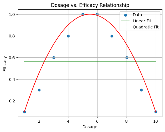
Neural network is one method to fit the non-linear relationship (Disclaimer: it can also be use in linear relationship data). The architecture of the neural network is consisted of input layer, hidden layer and output layer.

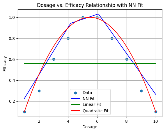
In the example above, I used a neural network with 1 input, 1 hidden and 1 output layer. In the hidden layer I used 20 nodes.

class SimpleNN(nn.Module):
  def __init__(self):
    super(SimpleNN, self).__init__()
    self.hidden = nn.Linear(1, 20) # 1 input node, 20 hidden nodes
    self.output = nn.Linear(20, 1) # 20 hidden nodes, 1 output node
    self.relu = nn.ReLU()       # Activation function

  def forward(self, x):
    x = self.relu(self.hidden(x))
    x = self.output(x)
    return x

Josh Starmer has a very good visual explanation of the process. Essentially, arriving at each node in the hidden layer, we take the input data, we multiply by the weight and add a bias term. Then at the node, we perform a function f(x’) on that number x’ we just derived. This function (refered to as activation function) can take many forms, such as sigmoid or rectified linear unit. Effectively, at each node at the hidden layer, we generate a curve of data. These “curves” of data take different forms, but when they are summed up together, they give us the curved/ bell shape line we see in the picture above.

Gradient descent

In linear regression, we can arrive at the best parameters/ coefficient of the equation using the closed form solution. For non-linear methods, we use a different approach, that in essence reiteratively finds the most optimal solution.

This is achieved by using the chain rule

Chain rule

Imagine you want to know what is the relationship between weights and shoe size. You know the equation for weights and heights, and heights and shoe size.

So \(Height = 3 \times Weight\) \(SSize = \frac{1}{4} \times Height\) *assuming the line passes through the intercept

From this, you can say that for every increase in weight, you gain 2 unit increase in height, and consequently for every increase in height, you have 0.25 unit increase in shoe size or \(\frac{dHeight}{dWeight} = 2\) \(\frac{dSSize}{dHeight} = \frac{1}{4}\) From here we can see the relationship between weight and shoe size, by replacing the terms in the original equations \(Height = \frac{dHeight}{dWeight} \times Weight\)

So for every increase in weight, there is 0.5 unit increase in shoe size.

This is what happens when the relationship is obvious (we see that height links weights to shoe size). In cases where this is not obvious, for example,

$SSize=\sqrt{Age^2+\frac{1}{2}} $

we can use the chain rule, to replace $Age^2+\frac{1}{2}$ with a different collective term, and use the chain rule to get the derivative of shoe size with respective to age.

Case 1. Find the most optimal intercept

In linear regression, the best coefficients (or the best fit line) are those that minimises the residuals (errors or difference in value) between the data point and its corresponding value on the fitted line. In other words, we want the line to be as close to the data point as possible.

Gradient descent is the algorithm that we can use to find the best slope and intercept.

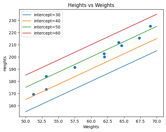
Suppose we have the following data point, and we want to find the best intercept. Here, we have plotted several intercept values. What we want is to find the line with an intercept, which give us the smallest sum of squared residuals (this is often referred to as the loss function). We can do this manually, by selecting an intercept value, e.g., 30, and then plug it into the equation we have, and then calculate the squared residual for each point of weight we have. The figure below show the sum of squared residuals we get at different intercepts values. This clearly shows that at intercept = 50, the sum of squared residual is the smallest.

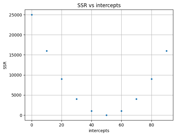
However, by doing so we are not guaranteed that we will see the most optimum solution and we don’t know how many values of intercept we need to try out. On the other hand, gradient descent will try out only a few values far from the global optimum, but more value as it gets closer to the optimum solution.

Step 1. We do this by just writing out the equation and expand it using the chain rule. \(\begin{align} SSR = \sum(observed-predicted)^2 \\ SSR = (y_1 - (a + b\times w_1))^2+...+(y_n - (a + b\times w_n))^2\\ \frac{dSSR}{da} = -2(y_1 - (a + b\times w_1))...-2(y_n - (a + b\times w_n))\\ \end{align}\)

where $a$ is the intercept and $w$ is the weight and $y$ is the observed height.

Step 2. Now instead of trying out multiple different intercept values, we can start with a random value, say 0. This will gives us the $\frac{dSSR}{da} = -1000$ at intercept.

Step 3. We multiply the slope at intercept = 0, with another value called a learning rate to give us a step size. Intuitively, slope and step size tell us the location of the next intercept value we must try. So in this example, because we want to find the point where $\frac{dSSR}{da}=0$, -1000 is still a long way away. If we set the learning rate to 0.01, then our step size is -10.

Step 4. The next intercept we want to try is $a’ = a - step size$. So the new intercept we try is -10. And we can repeat this until we are satisfied that we have found the minimum point or the number of attempts has been reached.

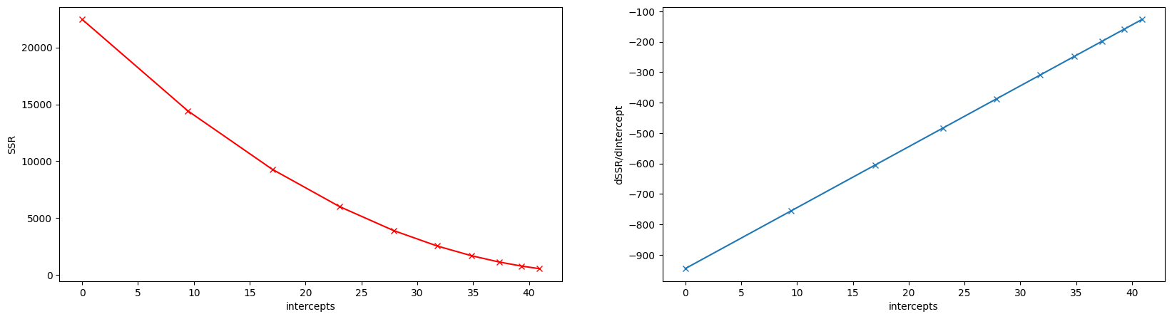
As you can see from the graph above, the interval between each successive intercept attempted becomes smaller as we get closer to intercept = 50.

Case 2. Find the most optimal intercept and slope

The solution is very similar to the previous case. Here, instead of just calculating the derivative of sum of squared residual with respect to the intercept, we are also calculating the derivative of the sum of squared residual with respect to the slope.

Next, we start with random starting value for both intercept and the slope, and we repeat the same steps as described above, updating the new intercept and slope after each step.

Example code:

np.random.seed(42) # for reproducibility
weights = 50 + 20 * np.random.rand(50) # weights between 50 and 70

# Define the intercept and slope
true_intercept = 0.4
true_slope = 2.5

# Calculate corresponding heights with some noise
# Adding a small amount of random noise to simulate real-world data
noise = 5 * np.random.randn(50)
def f(intercept,slope,weights,noise=None):
  if noise is None:
    y = intercept + slope * weights
  else:
    y = intercept + slope * weights + noise
  return y

def mse(y_obs, y_pred):
  return np.sum((y_obs - y_pred)**2) / len(y_obs)

heights_obs = f(true_intercept,true_slope,weights,noise=noise)

class GradientDescent:
  def fit(self,x , y, lr=0.0001, n_iterations= 1000):
    self.intercepts = [] # list of intercepts attempted
    self.slopes = []
    self.cost_functions = [] # list of cost_functions attempted
    self.derivative_intercepts = [] # list of derivatives of ssr wrt intercept
    self.derivative_slopes = [] # list of derivatives of ssr wrt slope
    n = len(x)
    current_intercept = 0.01
    current_slope = 0.01
    previous_cost = None
    for i in range(n_iterations):
      # step 1: calculate y_pred and cost function
      y_pred = f(current_intercept, current_slope, x)
      cost_function = mse(heights_obs, y_pred)
      # step 2: calculate the derivative and update the slope and intercept
      derivative_intercept = np.sum(-2/n*(heights_obs - y_pred))
      derivative_slope = np.sum(-2/n*(heights_obs - y_pred)*x)
      
      if previous_cost and abs(previous_cost-cost_function)<=1e-6:
        break
      previous_cost = cost_function

      # update the lists
      self.intercepts.append(current_intercept)
      self.slopes.append(current_slope)
      self.cost_functions.append(cost_function)
      self.derivative_intercepts.append(derivative_intercept)
      self.derivative_slopes.append(derivative_slope)

      current_intercept = current_intercept - lr * derivative_intercept
      current_slope = current_slope - lr * derivative_slope
    
    return current_intercept, current_slope

Output

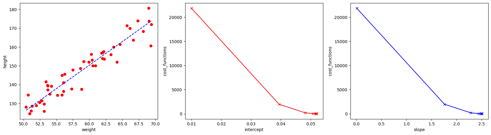
The cost function used here is mean squared error (basically just mean of the sum of squared residual). The middle and right-most figures indicate the change in the cost function at different intercept and slope. The estimated intercept (bias) and slope (weight term) are very close to the true values.

Backpropagation: Gradient Descent and Chain Rules on Steroid

From case 2, we can actually expand to include as many terms as possible (i.e., we can find the optimal solution for as many terms as we want, the example above is only for 2). Additionally, as we see above, we can update all of the terms simultaneously. Here, we follow the same steps, we calculate the derivative of the cost function with respect to the term, plug the random values to the equation, and then update the terms as you attempt to minimise the cost function.

Again, Josh Starmer made an amazing visual explanation of the backpropagation.

Rather than showing the math notation and the derivatives, I find it easier to understand when it is in the code form. Let’s take a neural network with the following architecture

1 input layer (2 neuron), 1 hidden layer (2 neurons) and 1 output layer (1 neuron).

In the forward pass.

import numpy as np
# --- Example Input data ---
X = np.array([[0.5], [0.1]])  # shape: (2, 1)
Y = np.array([[1]])           # shape: (1, 1)

# --- Activation function ---
def sigmoid(z):
    return 1 / (1 + np.exp(-z))

# --- Parameters ---
np.random.seed(42)
W1 = np.random.randn(2, 2)  # hidden layer weights
b1 = np.zeros((2, 1))       # hidden layer bias
W2 = np.random.randn(1, 2)  # output layer weights
b2 = np.zeros((1, 1))       # output layer bias

# --- Forward pass ---
Z1 = W1 @ X + b1              # shape: (2, 1)
A1 = sigmoid(Z1)             # shape: (2, 1)
Z2 = W2 @ A1 + b2            # shape: (1, 1)
A2 = sigmoid(Z2)             # shape: (1, 1) — final prediction y_hat

Here we defined the 3 layers. The input layer is of (m x n) dimension, where m is the number of data point, and n is the number of features we have (e.g., weights and heights). The hidden layer neuron in layer $L$ will have the dimension of (m x z) where z is the number of neurons defined in the $L$ layer (so in the example above, z = 2). The matrix W1, which is the weight of the hidden layer will have the dimension of (n neurons in previous layer, n neurons in this layer). Thus, as we pass our input data from the input layer to the hidden layer, we perform the following multiplication $ X \cdot W + b $. Subsequently, we use the sigmoid activation function. The point of the activation function is to introduce non-linearity. We do this until we get to the final output layer. Next we get the cost of this forward pass. We use the mean squared error as the cost function.

# --- Cost (MSE) ---
m = 1
cost = np.sum((A2 - Y) ** 2) / m

Using the cost, we can calculate which direction we need to update our weights and bias terms. Let’s start with the outer most layer.

def sigmoid_derivative(a):
    return a * (1 - a)

# --- Backward pass ---
# Output layer
dC_dA2 = 2 * (A2 - Y)                       # shape: (1, 1) m = 1
dC_dZ2 = dC_dA2 * sigmoid_derivative(A2)      # shape: (1, 1)
dC_dW2 = dC_dZ2 @ A1.T                        # shape: (1, 2)
dC_db2 = dC_dZ2                               # shape: (1, 1)

First, we calculate what is the derivative of cost with respect to W2.

and b2

Next, we moving the hidden layer (the preceding layer), which has 2 neurons.

# Hidden layer
dC_dA1 = W2.T @ dC_dZ2                        # shape: (2, 1)
dC_dZ1 = dA1 * sigmoid_derivative(A1)     # shape: (2, 1)
dC_dW1 = dC_dZ1 @ X.T                         # shape: (2, 2)
dC_db1 = dC_dZ1                               # shape: (2, 1)

Here, we again calculate the derivative of cost w.r.t. W1 and b1.

Finally, we can update W1, W2, b1 and b2 using the step size and learning rate

# --- Update weights ---
lr = 0.1
W1 -= lr * dC_dW1
b1 -= lr * dC_db1
W2 -= lr * dC_dW2
b2 -= lr * dC_db2

# --- Output ---
print("Cost:", cost)
print("A2 (prediction):", A2)
print("Updated W1:\n", W1)
print("Updated W2:\n", W2)

And this is one pass. We can repeat this multiple time until we cannot update the weights anymore or a threshold has been reach.