Transformers architecture and LLM
The full guide of huggingface is found here [1]. This is a review of the main concepts along with some codes.
Introduction
- Natural language processing (NLP) refers to the field focused on enabling computers to understand, interpret and generate human language.
- Large language models (LLMs) is a collective term of NLP models that are trained on a massive dataset. Models example are Llama and Generative Pretrained Transformers (GPTs).
Some NLP tasks include:
- Classifying the whole senteces - e.g., sentiment analysis
- Classifying individual word - e.g., named entity extraction
- Question and answering - given a question and context, extract a factually correct answer.
- Generating text content
- Translation
Development of LLMs also means that we can now have seemingly all-knowing chatbot. However, some of the problems associated with LLMs are:
- Hallucination - where the model will provide with ostensibly correct-sounding answer, that is in fact wrong.
- Bias
- Lack of reasoning
- Computational resources
Transformers
Transformers is a type of architecture that underlies many of the well-known NLP models. This video by 3Blue1Brown explains it quite well.
In a nutshell, a transformer is a deep neural network consisted of several layers, with each layer feeding information to the next. In the case of the GPT, a piece of text is fed to the transformer, and the transformer will output the next most probable word based on the input of all previous words.
The transformer library of huggingface is very versatile. For example, the pipeline object allows one to use a variety of pretrained models for different tasks, including:
text-generationtext-classificationsummarizationtranslationzero-shot-classificationfeature-extractionimage-to-textimage-classficationobject-detectionautomatic-speech-recognitionaudio-classificationtext-to-speechimage-text-to-text
The general code syntax is
from transformers import pipeline

classifier = pipeline("sentiment-analysis")
classifier("I've been waiting for a HuggingFace course my whole life.")
Output
[{'label': 'POSITIVE', 'score': 0.9925463795661926}]
from transformers import pipeline

classifier = pipeline("zero-shot-classification")
classifier(
    "Four legged animal with fur, and can be found mummified in egypt",
    candidate_labels=["dog","cat","chicken"],
)
Output
{'sequence': 'Four legged animal with fur, and can be found mummified in egypt',
 'labels': ['dog', 'cat', 'chicken'],
 'scores': [0.3621610403060913, 0.35874396562576294, 0.27909499406814575]}
Sometimes it doesn’t work as you expect
Transformers architecture
Transformers are language models, meaning they can be trained in a self-supervised manner. In a nutshell, self-supervised learning is a type of learning where the objective is computed from the input. For example, you crop a part of the image and you let the model predict that part of the image. In the case of NLP, this can be either predicting the next word after reading n numbers of words (causal language modeling), or predicting a masked input (masked language modeling). These are also known as auxiliary tasks or pretext tasks; you don’t really care about the performance of these tasks, but rather you use this as a pretext for the model to learn about intrisic relationship between the input data (e.g., semantic relationship between words or positions of the pixels within the image) [3]. These pretrained models are useful when are subsequently fine-tuned (using transfer learning) to a specific tasks.
Most of the transformers use the following three architecture: encoder-only, decoder-only or encoder-decoder (sequence to sequence).
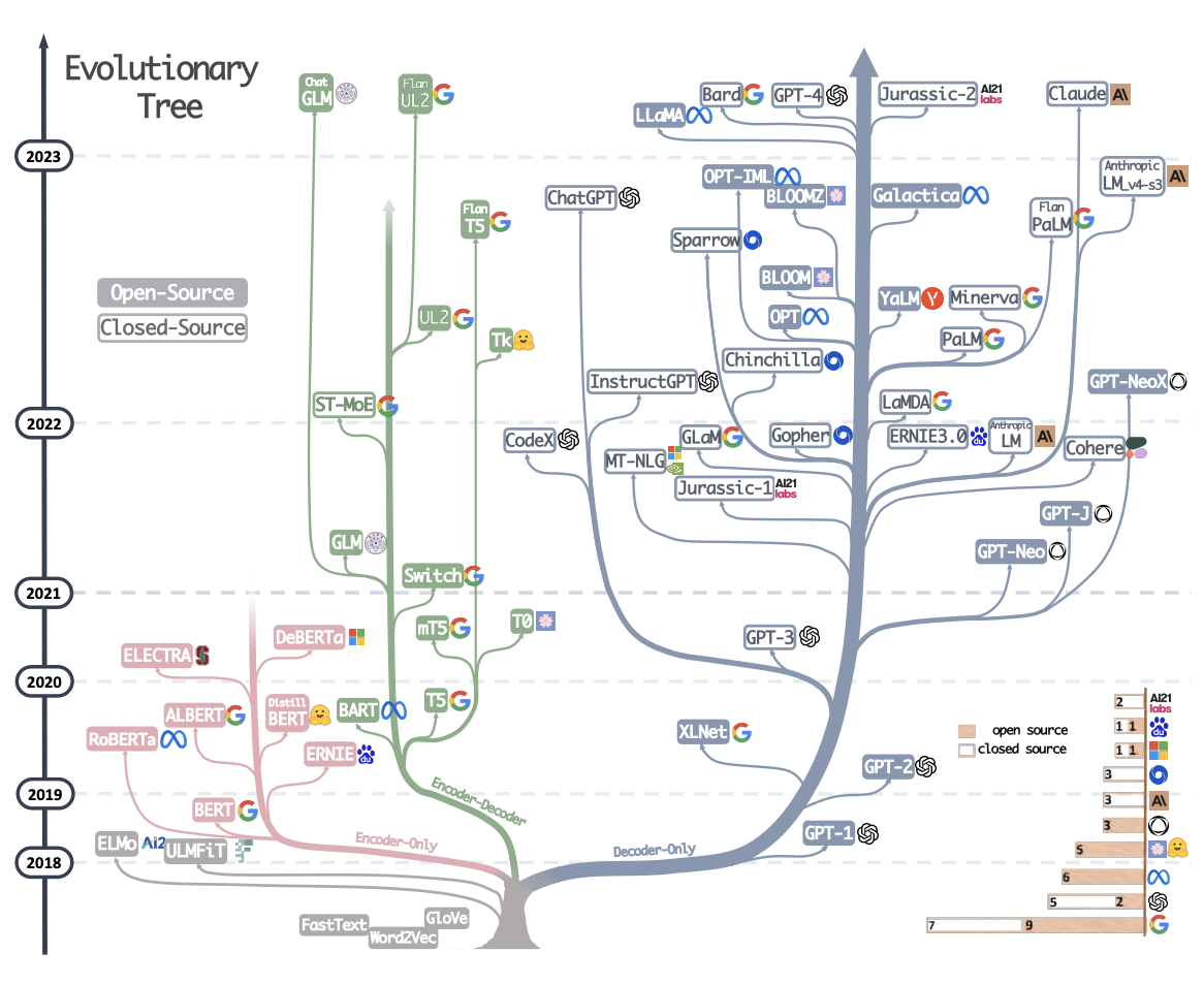 Image from Yang et al. 2023
In a nutshell, the difference between the three are as follows:
- Encoder only -> This type of model is useful when the task requires understanding the whole input. These models are characterised as having “bidirectional” attention, because the numerical representation of a word is “influenced” by the adjacent words on both side. This can be achieved by using a masked language modeling. These models are known as auto-encoding models. Encoder models are best suited for sentence classification, such as named entity recognition, and extractive question answering. Examples include BERT and DistilBERT.
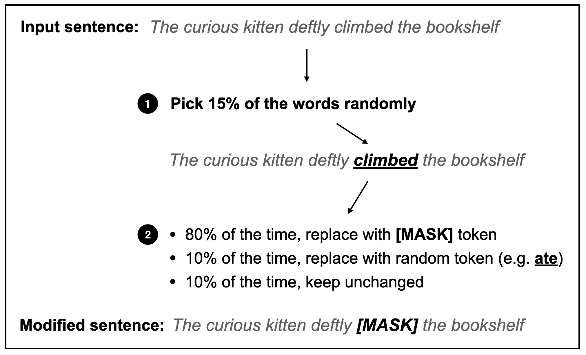
Example of masked language modeling. Image taken from Raschka, 2023
- Decoder only -> This type of model is useful when the task requires predicting the next word. These models are “unidirectional”, i.e., the only context the attention layer receives for a word comes from the words preceding it. This model is known as auto-regressive.
Modern LLMs mostly use decoder only architecture. Firstly, they are trained to predict the next token from the vast amount of data. Secondly, they are fine-tuned to a specific tasks. For example, text summarisation, question answering, code generation and so on.
- Encoder-Decoder -> This is the combination of the two. The input to the encoders are “converted” to numerical vector representation, which are then used as inputs to the decoder. The decoder in turn will use the information provided by the encoder and will generate the next token in the sentence.
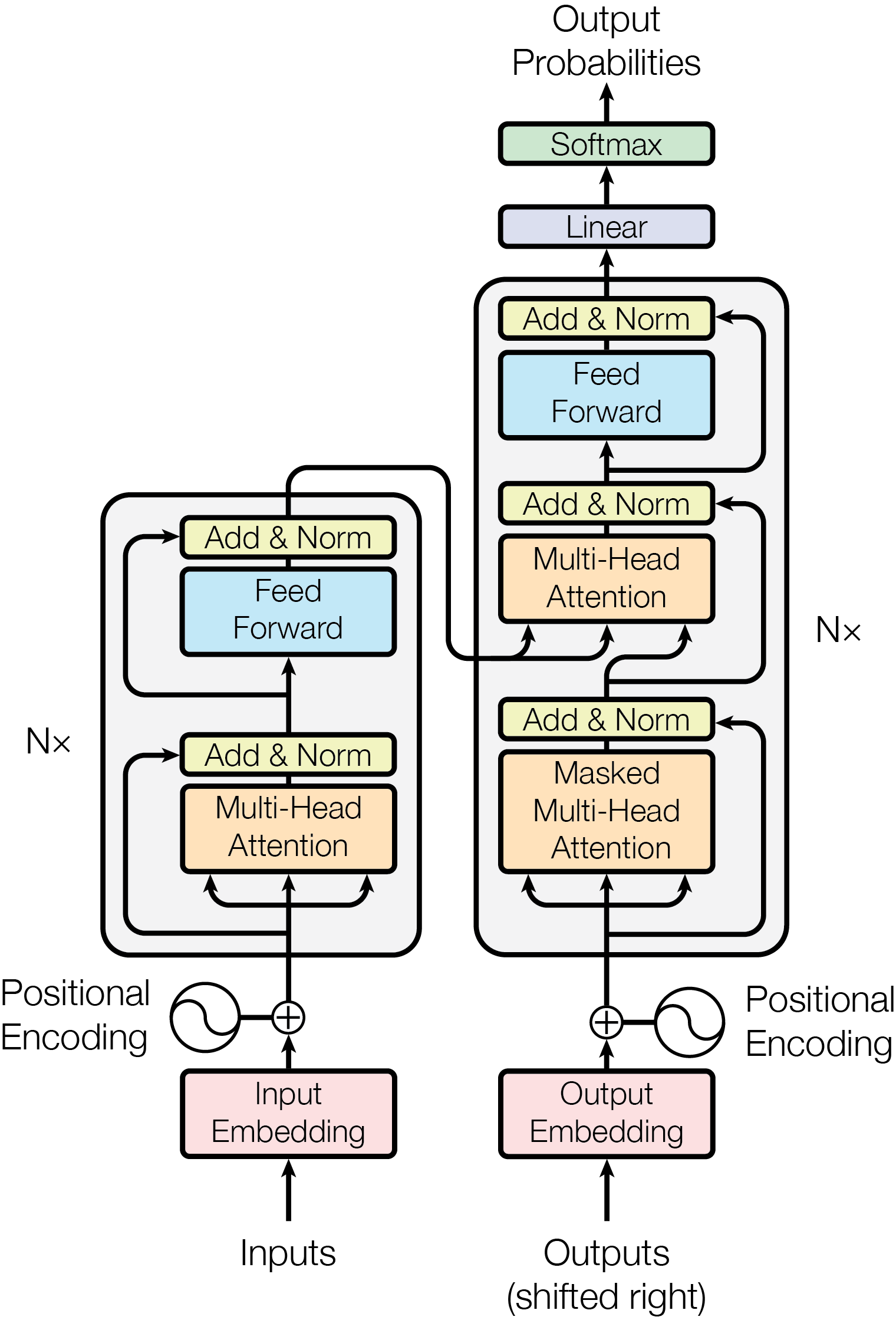
Illustration of taken from Vaswani et al., 2017
Best way to visualise this is in the translation tasks. If the sentence “Hi, my name is Hai” is fed to the encoder, the numerical representation will be added to the decoder along with a start sentence token. The decoder will then use the token and generate “Xin chào, tôi tên là Hải”, word by word until it receives a stop token. Example models are BART and T5.
The following table summarises the suggested architecture for each task. Taken from [4]:
| Task | Suggested Architecture | Examples |
|---|---|---|
| Text classification | Encoder | BERT, RoBERTA |
| Text generation | Decoder | GPT, Llama |
| Translation | Encoder-Decoder | T5, BART |
| Summarisation | Encoder-Decoder | BART, T5 |
| Named entity recognition | Encoder | BERT, RoBERTA |
| QA (extractive) | Encoder | BERT, RoBERTA |
| QA (generative) | Encoder-Decoder or Decoder | T5, GPT |
| Conversational AI | Decoder | GPT, Llama |
How does inference work?
Again, 3Blue1Brown explains it very well. Imagine each component in the neural network (weight) as a knob.
Inference is the process by which LLM generate the next word.
Attention
The attention mechanism is what gives LLMs their ability to understand context and generate coherent responses. Essentially, it allows words to have weights. For example, in the sentence “The capital of France is ….”, the words capital and France carry more weights than the rest.
The basic of the attention architecture
Consider these three sentences:
- Tower of Hanoi
- A collapsed tower
While it is the same word tower in both sentences, they carry a different meaning. The role of the attention network is to codify the “context” to the word “tower”. Or more generally, the attention network updates each word based on the presence of the surrounding words. This allows the LLM to generate a coherent and human-like text.
Let’s consider the following example, The quick brown fox jumps over the lazy dog (note, I will use the term token and word interchangeably). Before the training, each of these words is converted to an embedding vector, the -> E_1, quick -> E_2, brown -> E_3, fox -> E_4. The goal of the attention network is to update these vectors into E_1’, E_2’,…E_n’, such that they contain information encoded from the surrounding tokens. So more concretely, we want to the update the word fox, with the fact that it is quick and brown. In other words, a quick brown fox, would exist in a different position in the embedding space from fox.
Relevancy of the word
To update meaning of a token, we need to know which other tokens are relevant to it. In this example, quick is relevant to fox, but not lazy. One can ask the following question for each word, “Is there an adjective before this noun?”. If there is, then we want that adjective (quick) to influence more the meaning of that noun (fox) than words that are not relevant (e.g, the). In the attention network, this interrogation of relevancy between pairs of tokens is achieved via two sets of matrices, Query (W_Q) and Key (W_K).
Essentially, each one of the embedding vectors (E_n) is multiplied by a W_Q (query matrix) and W_K (key matrix) to generate a corresponding query vector (Q_n) and key vector (K_n). In the example above, each Q_n can be thought of as the corresponding token asking whether there is relevancy between it and the surrounding tokens. Conversely, each K_n can be thought of as the answer to that. Each Q_n and K_n exists in a Query/Key high dimensional space, and the ones that are highly similar (high dot-product) to each other would indicate high relevancy. In the example above, if Q_4 indicates the query posed by the token fox, K_2 - the key answered by the token quick, and K_1 - the key answered by the token the, then the dot-product between Q_4 and K_2 will be higher than that between Q_4 and K_1. Obviously, there is no way you can decode what does Q_n or K_n means, but the idea is that at the end of the matrix multiplication, you are left with a dot-product table, such that the words relevant to each other would have a high dot-product (similarity value) between the Query and Key value. This dot-product table is also known as an attention pattern. Softmax function is generally applied to the columns of the dot-product table to indicate the weight (contribution) of each token on that particular token. To summarise, at the end of this step, we have for each token in the text the contribution and influence of other words on that token.
So how to actually update the meaning of the tokens (i.e. how to update the meaning of the word fox to reflect the quick brown fox). The easy way is to use a third value matrix (W_V). In the simplest terms, if you take the embedding value, E_2, of the word quick and multiply it with the W_V you get a value vector (V_2), with which if you add to the embedding vector, E_4 of the word fox, you get the embedding value of quick fox. If you do the same to the embedding value, E_3, of the word brown and add the value matrix V_3 to the embedding value of quick fox, you get the embedding value of quick brown fox. The trick here is you multiply the V_n vector with the corresponding dot-product in the dot-product table. In this way, the value vectors of tokens relevant to the token of fox, would contribute more than the one that does not. Adding the original embedding values of each token to the weighted sums of these value vectors gives us the new updated embedding values.
This concludes a single attention layer.
The dimensions of the matrices
These three matrices are tuneable parameters in the transformer. The W_Q and W_K are n x m matrices, where m is the number of tokens in the embedding, and n is the number of query and key values. The value matrix is often represented as a linear product of two matrices, which are of similar sizes to that of the query and key matrices.
In multi-headed attention map, this architecture is repeated across multiple layers, with each layer having its own tuneable W_Q, W_K and W_V. This allows the LLM to learn and impart different ways the context can change the meaning of the token.
How do LLMs store facts?
In between the attention layers are multilayer perceptrons. These make up 2 third of the number of parameters in LLMs.
In simple terms, each one of the embedding vectors generated from the last step is then passed to a series of matrix multiplication operation (in parallel). So if the sentenec is “Michael Jordan is the GOAT”, the embedding representation of “Michael”, and “Jordan” is passed through several layers.
The first layer will put the original embedding vector to a higher dimension, the second layer introduces non-linearity to the vector and the third layer will put the vector to the original dimension.
The first and the third layer can be thought of as a series of questions. In the first row of the first layer, the question may be “does the name correspond to Michael Jordan” -> if yes, then the dot product is 1. And then if first column of the third layer is related to basketball, then the information of basketball will be added as the first neuron in the preceding layer is 1 (i.e., activated). This allows for information/ facts to be stored in LLMs.